In this post we will see how Frank-Wolfe (FW) algorithm (aka Conditional Gradient algorithm) can be generalized to nonsmooth problems (see here for the paper corresponding to this post). By nonsmooth we mean optimization problems with a nondifferentiable objective function.
Let us first review the traditional FW algorithm. FW is typically appropriate to solve $\min_{x\in \mathcal{C}}f(x)$ where $\mathcal{C}\subset\mathbb{R}^n$ is a compact convex set and $f$ is a smooth function. Given a starting point $x_o\in \mathcal{C},$ FW refers to the following algorithm:
Smooth Frank-Wolfe algorithm (FW)
- for $~t=1,2,\ldots~$ do
- $\quad \quad x_{t+1} \leftarrow (1-\alpha_t)x_t+\alpha_ts_t \quad \text{where} \quad s_t \in \arg\min\limits_{s\in\mathcal{C}} \nabla f(x_t)^Ts$
where $s_t$ is the (feasible) direction of update and $\alpha_t$ is the step size.
Convergence: We will just sketch the most basic convergence proof. There is a lot of work devoted to making the algorithm provably faster in specific cases, see here. If $f$ is linear, then we are done in one iteration by setting $\alpha_1=1$, yay! So for a nonlinear $f$, it turns out that in order to study the convergence aspects of the algorithm, it is useful to define a measure of linearity of the function. Let’s call it $C_f$, the curvature constant of $f$,
Definition:
$\quad \quad \quad \quad C_f:=\sup\limits_{x,y\in \mathcal{C},\alpha\in[0,1]} \frac{1}{\alpha^2}\left(f(y)-(y-x)^T\nabla f(x)-f(x) \right)$
Basically it measures how accurate the linear approximation is for a given function $f$ on the feasible set $\mathcal{C}$ but only along our update direction. We can show that this is, in fact, bounded by the diameter of $\mathcal{C}$ and the Lipschitz constant $L$ of $\nabla f$. One version of the convergence proof is based on the Wolfe dual and showing the duality gap is $ \epsilon>0$ for a sufficiently large $T$ polynomial in $1/\epsilon$. The only constant that appears in the iteration complexity is the $C_f$ mentioned above. This method is often called “projection-free” since it only uses Linear Optimization (LO) oracle compared to the usual Projected Gradient Descent (PGD) which executes quadratic Optimization oracle.
How does FW compare with PGD for smooth $f$?
As mentioned above, because of its simplicity, the per iteration complexity of FW is much smaller for many popular machine learning problems compared to PGD (see here for an excellent discussion).
Let us see a few other ways in which both the methods compare with each other:
Convergence rate for $\Delta_t:=f(x_t)-f^*\leq \epsilon$ accuracy (ignoring universal constants) for smooth convex $f$ with no further assumptions:
Here FW matches PGD for smooth problems, but it turns out that neither of the two is the fastest since Nesterov’s accelerated gradient method achieves $O(LD^2/t^2)$.
Strong Convexity: The convergence cannot be improved for FW by assuming strong convexity properties of $f$ with a simple example whereas for PGD it can be.
Affine invariance of LO oracle: From a simple check, we can see that FW method cannot also be sped up by a smart change of coordinate system.
Sparsity: FW type algorithms have an inherent sparsity in its iterates $x_t$. For instance, suppose $\mathcal{C}$ is a simplex or nuclear norm ball. LO corresponds to computing a basis vector or a rank one matrix, hence after $t$ iterations, $x_t$ will have at most $t$ nonzero entries or rank $t$. This has close connections with designing sublinear algorithms and coresets (approximating a set of points by a subset algorithmically).
The points two and three can be considered as weaknesses of FW but recent papers show linear convergence for many interesting applications where projections in PGD cannot be done in practice, see this for instance. Now we are ready to discuss our paper.
What about FW algorithms for nonsmooth $f$?
It turns out that FW method when $f$ is nondifferentiable is not well explored. I will first mention two main approaches that deal with this case and point out an issue with each of them which we try to address in our work:
1. Gaussian smoothing: Hazan & Kale proposed optimizing a smoothed version $\hat{f}_{\delta}$ of $f$ by sampling. This approach is simple, and straightforward to implement. The convergence result shown is the following:
where $K$ is a constant (that depends on $D,L$) and $d\in [0,3/4]$. In the online or stochastic setting (where the cost functions are sampled iid from some unknown distribution), they show that we can set $d=1/2$ giving us a regret bound of $O(1/\sqrt{t})$ which is great. But in the offline setting which is what we consider here, in the worst case, $d=0$ results in a constant additive error that does not go to $0$ as $t$ increases. We observed for the SVM datasets in our experiments, the method may be slow since it requires $t$ number of function evaluations at each iteration. Recall that PGD/SGD require zero function evaluations.
2. Simulating PGD: Another approach which is a hybrid of FW and PGD is shown here where the authors assume that an extra (additive) function $\omega$ is present in objective function with the following properties: (i) proximal operator can be computed efficiently for $\omega$, and (ii) subgradient of the convex conjugate of $\omega$ can be computed efficiently. They also present analysis showing a $O(1/\sqrt{t})$ convergence rate. We call this as “simulating” PGD since (other than some specific cases) proximal operators in general can be thought of as projection operators.
In our work, we
- do not do gaussian smoothing, and
- do not assume any additional functions so we call our method “deterministic”.
Of course, this comes at a price, our oracle (subproblems) becomes a bit more tricky and deals with subdifferentials and their relatives (which may be weird). We show that for many interesting problems this is not a big issue. We also perform empirical evaluations.
What will this give us?
We found empirically that gaussian smoothing is very slow both in wall clock time and #-iterations. Our algorithm is faster than CPLEX linear programming solver on the SVM datasets that we tried to solve in terms of wall clock time (excluding the preprocessing time). For all these problems, we explicitly bound the coreset size as well and show that our algorithm is (weakly) sublinear in the dataset size sense. At the end of this post, I’ll mention some open problems that we think are interesting in this direction.
Our approach
Since convergence of FW methods for smooth $f$ depends on the curvature constant $C_f$, the natural thing to do is define a quantity that is analogous for the nonsmooth case.
Can we try the subdifferential?
So we tried doing exactly that and replaced the gradient with subdifferential in the definition of $C_f$. Unfortunately, this does not work and I’ll give a simple 1D example. Let’s modify the definition of $C_f$ to $C_f^{\text{exact}}$ as,
Definition:
where $y=x+\alpha (s-x)$. Existence of a solution to the inner optimization problem for a fixed $x,s,\alpha$ follows from the fact that the subdifferential of a continuous convex function is a compact set. Now let $f(x) = |x|$ over $D=[-1,+1]$. For any $x\in (0,1/2)$, let $s = -1+x$ and $\alpha=2x$ which implies that $y=-x$. Then by definition,
where we used the fact that $\partial f(x)={1}$ since $f$ is differentiable at $x$ in the second equality. Taking limit as $x\to 0^{+}$, we have that $C_f^{\text{exact}} \geq \infty$ which implies that we cannot obtain a $C_f^{\text{exact}}$ that can upper bound this quantity for all $x\in (0,1/2)$. This example shows that linear approximations based on ordinary subgradients can be arbitrarily poor in the neighborhood of nonsmooth points. Intuitively, the subdifferential is a discontinuous multifunction and provides an incomplete description of the curvature of the function in the neighborhood of the nonsmooth points. We show that this can be fixed by using what is called as the $\epsilon-$subdifferential which is also multifunction but is continuous (say in the measure sense) defined as,
Definition:
Setting $\epsilon=0$ gives us the usual subdifferential. $\epsilon-$subdifferentials are scary: assume $f=\sum_i f_i,$ where $f_i$ is convex. Then we have that,
We can see that, this set is huge compared to the usual subdifferential. See here for a formula for supremum of finite linear functions aka piecewise linear functions. We then found out that it is enough if we work instead with $T(x,\epsilon)$ defined as,
Definition:
where $N(x,\epsilon)$ is a neighborhood containing $x$. Basically, if we are close to a nonsmooth point, then we should also take into account the “derivatives” of that point. $T(x,\epsilon)$ is very intuitive to understand, also it keeps easy problems easy since if the neighborhood of the current point is smooth, then the gradient is good enough. This aspect is unique to our work to the best of our knowledge.
The oracle: LO oracle as we saw is very weak to provide the necessary convergence, so we use $T(x,\epsilon)$ instead. We now specify the comparison of the oracles (or subproblems solved in each iteration) that we use and the one used for the smooth case, given $x\in\mathcal{C}$, compute $s\in\mathcal{C}$ such that
and the corresponding curvature quantity that we have to bound is naturally defined as,
Definition:
$\quad \quad \quad \quad C_f(\epsilon):= \sup\limits_{x,s\in \mathcal{C},\alpha\in[0,1]}\left( \min\limits_{d\in T(x,\epsilon) } \frac{1}{\alpha^2} \left( f(y)-f(x)- \langle y-x,d\rangle\right)\right)$
where $y=x+\alpha(s-x)$ as before. Hand waving a little, note that if there are say $m$ nonsmooth points, then at most $n$ convex optimization problems are solved at each iterations and hence the subproblems are efficiently solvable, this is the case with many problems like SVMs, Graph Cuts, Sparse PCA,$1-$median etc..
Convergence: Assuming that $C_f(\epsilon)$ is bounded, the convergence proof is similar to that of the smooth case however there is a small catch: we arrive at a recursion of the following form using simple algebra, let $h(x)=f(x)-f^*$ and $C_f(\epsilon)\leq \frac{D_f}{\epsilon}$,
Now we make an observation. In the smooth FW, the power of $\alpha_k$ in the second term is $2$ instead of $3/2$ here. Choosing the standard step size sequence of $2/(k+2)$, we can show convergence of the algorithm but the rate gets slowed to $O(1/\sqrt{t})$ from $O(1/t)$ as in the smooth case which is reminiscent of the classical PGD. In the rest of the paper, we show that $C_f$ is indeed bounded for those problems. In the table we show the list of the problems that we considered in our paper and their bounds:
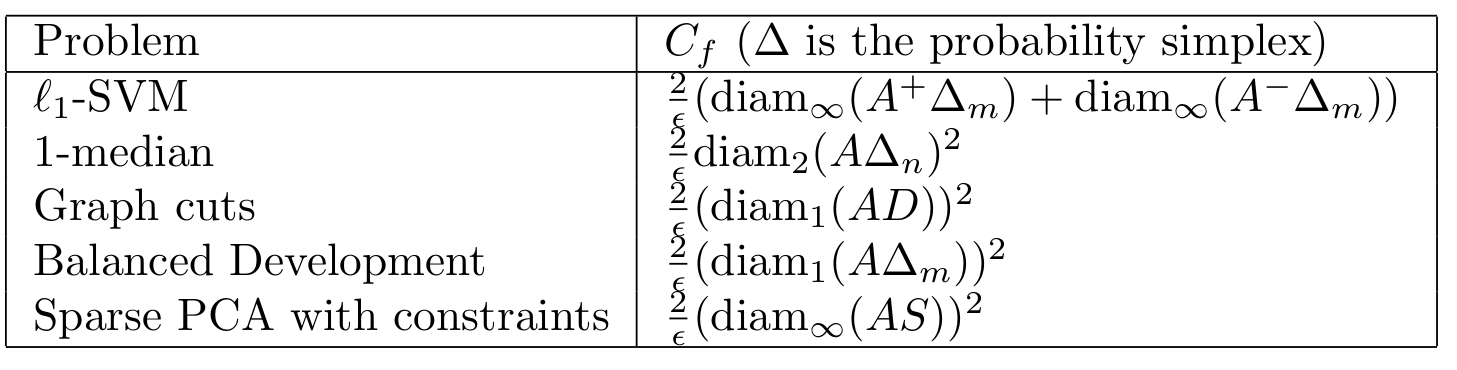
To prove the $C_f$ bounds, we choose an appropriate neighborhood for each problem, hence the diameter is measured with different norms. The proof gets a bit technical with the computation of the mentioned subdifferentials.
Let us see if the bounds are any good. Let’s consider the case of $\ell_1$-SVM. Assume that the positive and negative labeled instances be generated by a gaussian distribution with mean $0$ and $\mu$ respectively and variance $\sigma I$. Then we have that,
using the properties of maximum of sub-gaussians. This shows that the dependence of $C_f$ is logarithmic in the dimensions. Similarly we will get $\sqrt{n}, n\log n$ for $\ell_2,\ell_1$ norm diameters respectively showing that the $\mathbb{E}C_f$ is near linear in the dimensions which explains the impressive empirical performance of our algorithm.
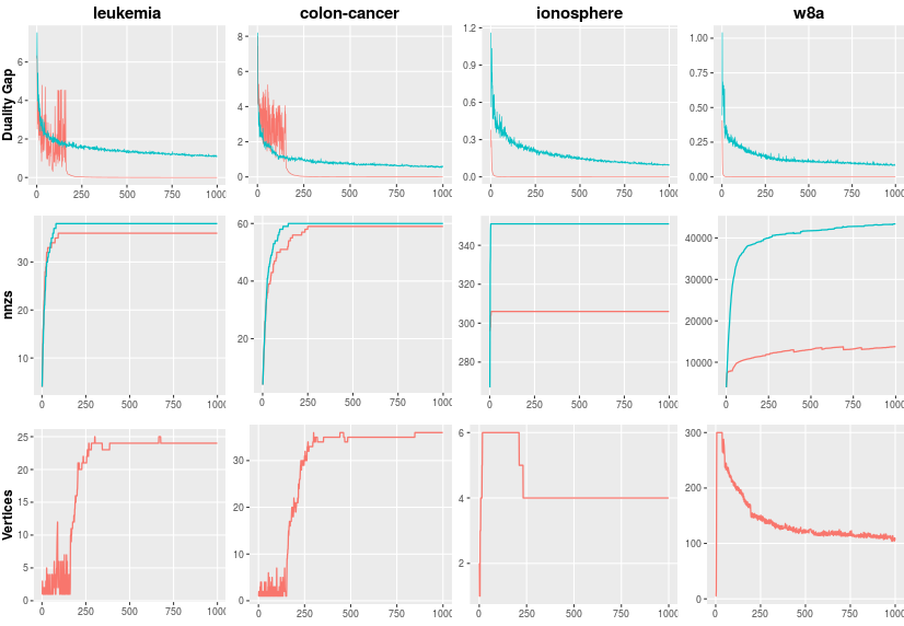
I did not talk much about the coreset (measured in terms of number of nonzero elements (nnzs) in the figure) aspect in this post but we see that the nnzs of our algorithm maintains sparse iterates compared to the gaussian smoothing approach. Please see our paper for more details on how we bound nnzs. Vertices measure the number of nonsmooth points, as we can see, they decrease as iterations (recall $\epsilon_k=\sqrt{\alpha_k} $).
Open problems: There are many problems that I think are interesting in this area. First, can we fully characterize the efficiency of the oracle that we use in our algorithm? Second, can we use randomization to speed up the algorithm ignoring the extreme cases? This seems like it is related to average case analysis. Third, say we are at a point whose neighborhood which contains a nonsmooth point, can we ignore it and just use the gradient at the current point hoping that things will be fine probabilistically? Finally, can we bound the number of convex problems that one would expect to solve at each iteration? This should depend on the objective function, but what specifically seems like a harder question to answer. Even a measure theoretic argument I believe will be worthwhile to investigate since the number of nonsmooth points depends on the choice of $\epsilon_k=\sqrt{\alpha_k}$ which is diminishing suggesting that we are more likely to solve computationally harder problems in the early phases of the algorithm.
Main takeaway
We showed that for many popular nonsmooth problems in ML, there is a FW algorithm that produces a “coreset” or equivalently that there is an algorithm that provides an $\epsilon-$approximate solution using only sublinear data points.